Demo and Results
Video Demo
Pictures
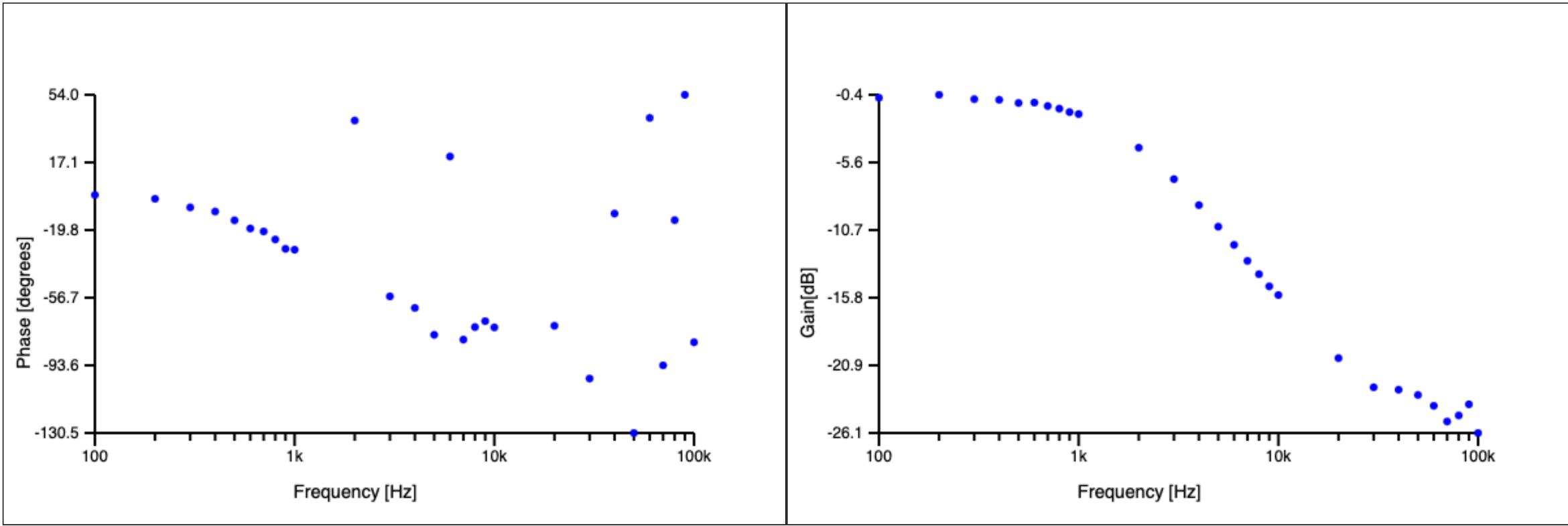
Figure 1 shows bode plots generated from a low pass filter. We can see the gain go from about 0 to -26 dB with a corner frequency at about 1 kHz.
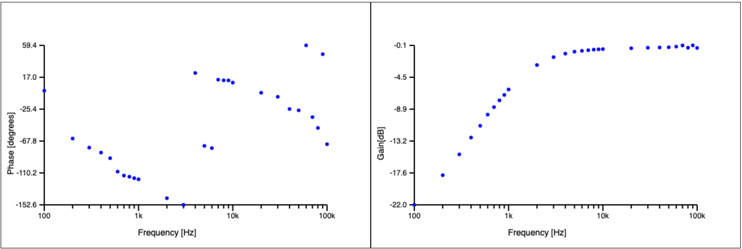
Figure 2 shows bode plots generated from a high pass filter. We can see the gain go from about -22 dB to about 0 dB with a corner frequency at about 1 kHz.
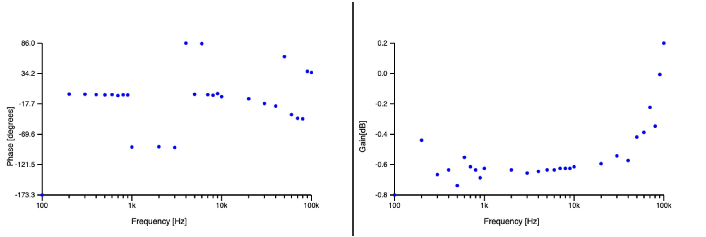
Figure 3 shows bode plots generated from just a thorugh wire. We can see the gain stay right around 0 which is what we would eexpect.

Results
Ultimately, we were able use the FPGA to drive an external DAC with a sine wave frequency sweep. The frequency sweep accurately ranged from 100 Hz to 100 kHz in order to cover three decades of information for the bode plot. We were also able to sample data using the MCU up to a frequency of 1 MHz. Finally, we were able to generate and display relatively accurate bode plots on a webpage. The gain is very consistent and is able to plot -20dB well for a simple first order filter. The phase struggles to keep up at high frequencies and is prone to outliers. However as seen in Figure 4, when connected to the through or wire with zero load the phase is very close to zero. As frequency increases the variability or error increases as the period of the wave decreases giving the phase extraction algorithm less time to react and sources of error such as propogation delay due to the instruction processing time impact the calculation more. Past 1 kHz the phase degrades to about 17% to 30% error on data points that are not outliers.